A rotary encoder is a transducer: it converts mechanical rotation into an electrical signal that a motion controller can use for position, velocity, and direction feedback. The conversion mechanism (the physical principle that translates rotation into electricity) determines the encoder’s accuracy, resolution, environmental immunity, and installation constraints.
Three physical principles are used in industrial rotary encoders:
- optical (with transmissive, reflective, or interferential variants),
- inductive (PCB-trace coils), and
- capacitive (electric field modulation
Each generates a periodic signal as the scale rotates relative to the sensor.
The Core Architecture: Sensor and Scale
All rotary encoders, regardless of sensing principle, consist of two functional elements:
- Scale (rotor): Attached to the rotating shaft or element whose position is measured. Carries the periodic pattern that generates the position signal.
- Reader (stator): Stationary. Contains the sensing electronics that detect the scale pattern and convert it into electrical output.
The critical interface between these two elements is the gap, the physical space through which the sensing signal must pass. Optical systems require a clear optical path across this gap. Inductive and capacitive systems transmit their signals through electromagnetic fields that are unaffected by most non-conductive foreign matter.
Optical Rotary Encoders: Sensing by Light
Transmissive Architecture
In transmissive optical encoders:
- An LED illuminates the scale from one side.
- The scale carries alternating transparent and opaque lines (50/50 duty cycle).
- Photodetectors on the opposite side of the scale detect the varying light intensity as the scale rotates.
- Two photodetectors separated in phase generate two sinusoidal signals in quadrature (90° phase offset).
The sinusoidal output enables interpolation, mathematical subdivision of the grating period into smaller position increments. At a grating pitch of 20 µm, a × 4,000 interpolation factor yields 5 nm position resolution.
Interferential Architecture
Interferential encoders use coherent laser light (typically vertical cavity surface emitting laser) and a grating that diffracts the incident beam.
The diffracted beams interfere with each other, creating an interference pattern on the detector. As the scale moves, the interference fringes shift across the detector array.
The detector captures the fringe phase shift as a sinusoidal signal. Because the measurement is based on the phase of the interference pattern rather than simple shadow counting, interferential systems can achieve resolutions of 1 nm or less on a 20 µm pitch grating, a ×20,000 or higher interpolation factor.
Key advantage of interferential over transmissive: The sinusoidal signal quality (signal-to-noise ratio, harmonic distortion) is higher for interferential systems, enabling higher interpolation ratios and better positional accuracy. The scale can also be metal tape (laser-etched) rather than glass with chromium lines, enabling longer linear scales and more flexible installation.
Absolute vs. Incremental Optical Output
An incremental optical encoder generates a periodic signal (A and B quadrature, with Z index). Position is accumulated by counting edges. For absolute position, a second sensor reads a pseudo-random pattern on the scale, a spatial sequence that is unique at every angular position. On power-up, the system reads this pattern and establishes absolute angular position without motion.
Inductive Rotary Encoders: Sensing by Electromagnetic Coupling
Inductive encoders use PCB-trace coils as both excitation and receiver elements.
The stator PCB carries excitation traces driven at 1–10 MHz. The rotor carries conductive targets (also PCB traces or metal patterns) that modulate the coupling between stator traces as the rotor rotates.
Secure Your Components Stock Now with Torquety
Reliable automation components for high-performance applications.
No line-of-sight requirement: The electromagnetic coupling between stator and rotor occurs through the gap regardless of non-conductive matter in the gap. This makes inductive encoders immune to dust, oil, water, and condensation that would disable optical systems.
Resolver comparison: Resolvers use the same inductive principle but implement the windings as physical wire wound on a core. Inductive encoders implement equivalent functionality using PCB traces, lower cost, smaller form factor, direct digital output without requiring a resolver-to-digital converter.
Resolution range: Up to 22 bits (approximately 4 million counts per revolution) at accuracy levels of approximately ±19 arc-seconds for high-performance inductive designs.
Capacitive Rotary Encoders: Sensing by Electric Field Modulation
Capacitive encoders measure the angular variation in capacitive coupling between stator and rotor electrode patterns. As the rotor rotates, the overlap area between stator excitation electrodes and rotor coupling elements changes sinusoidally, producing an output proportional to angle.
Holistic measurement: Advanced capacitive designs integrate measurements across the full disc area rather than at discrete points. This averaging provides inherent tolerance to localized anomalies (contamination, surface defects) and relaxes installation tolerance requirements.
No magnetic elements: Capacitive encoders are immune to external magnetic fields and generate no magnetic signature, relevant for applications near magnetometers or MRI systems.
Accuracy class: The best capacitive angle encoder designs achieve ±0.001° (±3.6 arc-seconds) accuracy, comparable to interferential optical systems.
Signal Processing: From Sine Waves to Position Data
Interpolation
The raw sensor output (whether from optical, inductive, or capacitive sensing) is a sinusoidal signal with a period equal to the grating pitch. Position resolution is increased by interpolation: subdivision of the grating period using the arctangent of the sin/cos ratio.
Resolution formula: Position resolution = grating period / interpolation factor
For a 20 µm pitch grating with ×4,000 interpolation: 20 µm / 4,000 = 5 nm resolution.
Accuracy vs. Resolution
Resolution and accuracy are not the same quantity:
- Resolution: The smallest position increment the encoder can detect (determined by interpolation)
- Accuracy: The maximum deviation between the actual position and the reported position (determined by grating uniformity, interpolation error, and thermal effects)
A high-resolution encoder with poor grating uniformity will report position with fine granularity but with large systematic errors. For precision applications, both resolution and accuracy must meet the application requirement.
Output Signals
Depending on the encoder design and application:
| Output Type | Format | Use |
|---|---|---|
| Incremental quadrature | A/B square waves + Z index | Velocity/position accumulation |
| Sin/cos analog | 1 Vpp differential sinusoids | High-resolution interpolation |
| Absolute digital | Serial word | Absolute position, power-up |
| Absolute digital | Parallel serial | Compact interface |
The Importance of ABZ for Absolute Encoders
In many implementations, absolute encoders output both a serial absolute position value and an incremental ABZ quadrature track simultaneously. The serial absolute value establishes position at power-up; the ABZ track provides high-speed incremental feedback during operation that the controller processes at full loop bandwidth without waiting for serial communication cycles.
Eccentricity: The Most Common Installation Error
Eccentricity occurs when the center of the encoder scale disc is not exactly aligned with the axis of rotation. This produces a systematic position error that repeats once per revolution.
Angular error due to eccentricity:
Angular error (radians) = arctan(eccentricity / radius).
For a 50 mm radius scale (100 mm diameter) with 25 µm eccentricity: Angular error = arctan(0.025 / 50) = arctan(0.0005) ≈ 0.0286° = 103 arc-seconds.
This error is beyond the specification of most precision encoders. To achieve ±2 arc-second accuracy on a 50 mm scale, eccentricity must be below approximately 1 µm — a precision that requires tooling marks on the hub or laser alignment.
Two-readhead compensation: Mounting two readheads at 180° on the same scale averages out the eccentricity error. If both readheads are at 180° apart, the positive eccentricity error from one readhead coincides with the negative eccentricity error from the other, and the average of the two readings is free of first-order eccentricity error.
For further reading, we highly recommend checking out Rotary Encoders for SATCOM Antenna Pointing Systems: Requirements and Technology Selection, as well as our articles on Slip Ring Offshore Wind: Corrosion Protection, Ingress Rating, and Lifecycle Service and Motor Temperature Monitoring in Servo Systems: Thermistor-Based Analog Sensing with Steinhart-Hart Coefficients.
Need a Custom Component Solution?
Contact our engineering team to discuss your application requirements and get a custom quote.